5 Working on an HPC

Now that you are more comfortable with the command line, we will learn how to work on the UVA Crunchomics HPC. In this section, you will go through the following steps:

Connect to the HPC and transfer your sequencing files
Install software using conda
Learn how to run analyses using SLURM job submission scripts
- srun for shorter interactive analyses
- sbatch for longer running, more resource intensive analyses

5.1 Connecting to the HPC

5.1.1 `ssh`: Connecting to a sever

SSH (Secure Shell) is a network protocol that allows you to securely connect to a remote computer such as the Crunchomics HPC. The general command looks like this:

ssh -X username@server

Here:

username is your account name on the HPC, i.e. your UvanetID
server is the address of the HPC you want to connect to, for Crunchomics this is omics-h0.science.uva.nl
-X enables X11 forwarding, which allows graphical applications from the server (like plotting or viewing images) to appear on your local machine. “Untrusted” X11 forwarding means the server can send graphical output, but it has limited access to your local machine

To log into the Crunchomics at UVA, use the following and enter your UvA password when prompted:

ssh -X uvanetid@omics-h0.science.uva.nl

Important

Important tips for connecting:

If you want to log into Crunchomics while working from UvA use the eduroam network, not the open Amsterdam Science Park network
If you are connecting from outside UVA, you must be on the VPN. Contact ICT if you have not set it up or encounter issues
Always double-check your username and server address to avoid login errors

5.1.2 Crunchomics: Preparing your account

If this is your first time using Crunchomics, you need to run a small Bash script to set up your account. This script will:

Add /zfs/omics/software/bin to your PATH variable. This basically allows Bash to locate and use the system-wide installed software available on Crunchomics
Set up a Python 3 environment with some useful Python packages pre-installed
Create a link to your 500 GB personal directory inside your home directory, giving you plenty of space to store data and results

To set up your account, run the following commands:

# First orient yourself by typing 
pwd 
ls -lh 

# Run the Crunchomics installation script
/zfs/omics/software/script/omics_install_script

# Check if something changed
# You now should see the personal folder inside your home directory 
ls -lh

5.1.3 `conda`: Setting up your own software environment

Many bioinformatics tools are already installed on Crunchomics, but sometimes you’ll need additional ones (like NanoPlot for analysing long-read data). To manage and install your own tools, we use conda/mamba, an environment manager that lets you create isolated environments for different software.

5.1.3.1 Install conda/mamba

Many systems already include conda or mamba. Before installing a new copy, check if it’s already available:

which conda
which mamba

If one of these commands returns “command not found”, then you can follow the next steps to install conda/mamba yourself. If you already have conda but not mamba that is fine, just replace all instances of mamba in this tutorial with conda.

If you don’t have access to either conda or mamba then you can install Miniforge (which includes conda and mamba by default) by running the following two commands:

# Download the miniforge installation script
curl -L -O "https://github.com/conda-forge/miniforge/releases/latest/download/Miniforge3-$(uname)-$(uname -m).sh"

# Execute the miniforge installation script
bash Miniforge3-$(uname)-$(uname -m).sh

During installation:

Read the license (scroll by pressing enter) and say “Yes” when asking for confirmation
Choose the installation location
- Important: On Crunchomics, your home directory has only 25 GB of space. Therefore install everything into the personal folder that comes with 500 GB: /zfs/omics/personal/uvanetID/miniforge3
Say “yes” when asked if conda should be initialized
Restart your shell by typing source ~/.bashrc. You now should see a (base) in front of your prompt indicating that you are now inside conda’s base environment
Verify the installation:

conda -h
mamba -h

5.1.3.2 Installing NanoPlot

NanoPlot is a visualization tool for long-read sequencing data. We can install it, and other software, using mamba (or conda if mamba is unavailable).

# Check if NanoPlot is already available
NanoPlot -h

# If not installed, create a new environment called nanoplot and install it
# Press "Y" when prompted about confirming the installation
mamba create -n nanoplot -c bioconda nanoplot

# Activate the new environment
conda activate nanoplot 

# Check if the tool is installed
NanoPlot -h

# Exit the environment
conda deactivate

Recommendations:

Whenever possible, use mamba instead of conda, it resolves dependencies faster
Keep your base environment clean (the base environment is the conda environment you start with when you log into the HPC). Always create new environments for each tool (conda create -n toolname …) instead of installing everything in base
Check the tool’s documentation for specific installation notes or version requirements
You can install specific versions when needed with mamba create -n nanoplot_v1.42 -c bioconda nanoplot=1.42
You can remove environments you no longer need with conda env remove -n nanoplot
You can list all existing environments with conda env list

5.1.4 Preparing your working directory

Next, you can start organizing your project folder. You always want to generate project folders inside your personal directory, which provides more storage than the home directory:

# Go into the personal folder
cd personal 

# Make and go into a new project folder
mkdir data_analysis
cd data_analysis 

# Ensure that you are in the right folder 
pwd

You now have a clean workspace for all the analyses that you will run during this tutorial on Crunchomics. As in your local machine, it’s good practice to keep your raw data, results, and scripts organized in separate folders.

5.1.5 `scp`: Transferring data from/to a server

To learn how to transfer data to Crunchomics, we want to transfer the data folder (the one you have generated in previous part of the tutorial) to the HPC. We can do this with the scp(Secure Copy Protocol) command, which securely transfers files or directories between your computer and a remote server.

The basic syntax is:

scp [options] SOURCE DESTINATION
For connecting to any HPC the syntax is server:file_location

When transferring data you must run the command from a terminal session on your own computer, not from a terminal session that runs on the HPC. To keep yourself organized its often useful to have one terminal session open on your laptop and another one Crunchomics as shown in the example below:

To copy the entire data folder into your Crunchomics project folder, use:

# Run this from your local terminal (not while logged into the HPC) 
# Run this while being inside the data_analysis folder to be able to access the data folder
# Replace 'username' with your UvAnetID
scp -r data username@omics-h0.science.uva.nl:/home/username/personal/data_analysis

# Run this command while being logged into the HPC
# and while being inside the data_analysis folder
# to check on the HPC that the files arrived:
ll data

Notes:

The -r option copies directories recursively, i.e. you want to copy everything in the directory and the directory itself (recursively)
It’s helpful to keep two terminal windows open: one for your local computer and one for the HPC
Run this command from inside your local data_analysis folder (the one you created earlier)

Tip: Moving data from the HPC to our own computer

You can also move results from the HPC to your computer. For example, to copy a single genome file from Crunchomics:

scp username@omics-h0.science.uva.nl:/home/username/personal/data_analysis/data/LjRoot303.fasta .

Here, the . at the end means “copy to the current directory” on your local machine. If you want to copy to another location, replace . with a path.

5.2 Submitting jobs with SLURM

In the HPC introduction, you learned that there are two main “sections” on an HPC:

Login node: where you log in and do light work, such as moving files, editing scripts, or preparing jobs.
Compute nodes: where the actual analyses run. These nodes have more CPUs and memory and are managed by a scheduling system.

To use these compute nodes efficiently, we communicate with them through SLURM, a workload manager that decides when, where, and how your jobs run based on the available resources.

5.2.1 `squeue`: View info about jobs in the queue

The command below shows you which jobs are currently running or waiting in the queue:

squeue

This displays all jobs submitted to the system, and might look something like this:

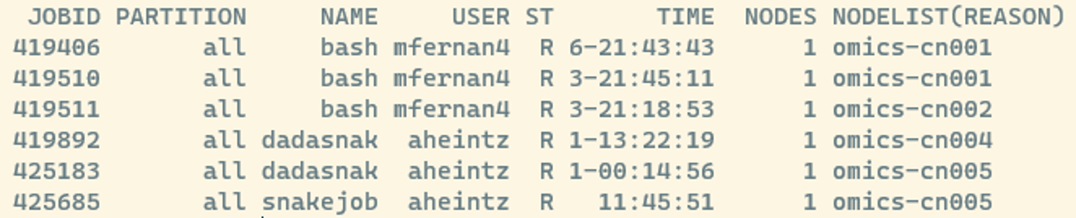
Some useful columns to know:

JOBID: a unique number assigned to each job; you can use it to check or cancel a job later.
ST: the current state of the job (e.g., R = running, PD = pending).
A full list of SLURM job state codes can be found here

If you have already submitted a job, it will appear in this list. To see only your own jobs, you can add the -u flag followed by your username or the USER variable:

squeue -u $USER

5.2.2 `srun`:Submitting a job interactively

Now that we’ve seen how to check the job queue, let’s learn how to actually run jobs on the compute nodes. There are two main ways to submit jobs: srun and with sbatch. We’ll start with srun, which you typically use when:

You want to run tasks interactively and see the output directly on your screen
You are testing or debugging your commands before writing a job script
You have short jobs (usually less than a few hours)

Important: Jobs started with srun will stop if you disconnect from the HPC (unless you use tools like screen or tmux, which we won’t cover in this tutorial).

Let’s start with a very simple example to see how srun works:

srun --cpus-per-task=1 --mem=1G --time=00:10:00 echo "Hello world"

Here’s what each part means:

srun → communicate to SLURM that you want to run something on the compute node with the following resources:
--cpus-per-task=1 → request 1 CPU core
--mem=1G → request 1 GB of memory
--time=00:10:00 → set a maximum runtime of 10 minutes
echo "Hello world" → the actual command to run (echo is a command that prints text to the screen)

So the arguments after srun and before echo are where you tell SLURM what resources to allocate on the compute node. Note, that after running this command that you might see Hello world twice. This is fine and just some specific behavior of some HPC systems we don’t need to worry about.

5.2.3 Running a analysis with Seqkit interactively

Next, let’s use srun for something more useful. We will analyze the fasta files that we have explored using seqkit, a fast toolkit for inspecting FASTA/FASTQ files. Seqkit comes with different modules, for example the stats module, that generates basic summary statistics from sequence files and can be called with seqkit stats.

Tip: Whenever you use a tool for the first time, check its help page (e.g., seqkit -h) to see all available options or check online for a manual or basic usage information.

# Create a results folder with a seqkit folder sinide
mkdir -p results/seqkit 

# Run seqkit with srun
srun --cpus-per-task=1 --mem=5G seqkit stats data/*fasta -Tao results/seqkit/16s_stats.tsv --threads 1

# View the results (press 'q' to exit less)
less -S results/seqkit/16s_stats.tsv

Here:

seqkit stats data/*fasta → Use the seqkit stats module to analyse all FASTA files in the data folder ending in fasta
-Tao → options to store output in tabular format (-T), include all stats (-a), and write to file (-o)
--threads 1 → run on one thread (should match --cpus-per-task=1)
- Important: Whenever you submit jobs to the compute node, make sure that the number of requested CPUS/threads match with the number of CPUS used by the software
The results are stored in results/seqkit/16s_stats.tsv

This job runs very quickly, so fast that it might not even appear in the queue when you type squeue.

When you open the results file, you will, among others, see:

The number of sequences in each fasta file (num_seqs), this should match with what you saw during the CLI tutorial part
The average length of the sequences in bp (avg_len)
Additional metrics such as the minimum, maximum or total sequence length

Tip: Choosing the right amount of resources

When starting out, choosing the right amount of CPUs, memory, or runtime can be tricky. Here are a few rules of thumb:

Start small, a lot of tools don’t need huge resources for small test runs
Check the tool’s documentation, some might list recommended resource settings
When starting out, you can begin by testing on a subset of your data first. It runs faster and helps you debug
If your job fails or runs out of memory, increase the resources gradually
Once you have a stable workflow, you can scale up

Remember: Over-requesting resources can make jobs wait longer in the queue — and can block others from running.

Tasks

Now it’s your turn to run an srun job interactively by exploring the FASTQ files that you have generated during your practical. Follow these steps:

Task 1: Inspect the data

Without uncompressing the FASTQ file, explore the content of the FASTQ files by viewing the first few lines of barcodeX.fastq.gz using zcat and head. Replace barcodeX with the barcodeID that you prepared during the practical.

You can get the FASTQ file as follows:

If you are following the Microbial Ecology course:

If you have prepared more than one barcode during the practical then check the individual file sizes of your barcodes and find the barcode with the largest file size. You will analyse this sample throughout this tutorial to keep things simple. Throughout this tutorial replace barcodeX with that barcode ID.

If want to know how to analyse several samples in an efficient manner, you can have a look at an example workflow after you are done with the full tutorial.
```
# Check the file size of all barcodes 
ls -lh /zfs/omics/projects/education/miceco/data/practical/*.fastq.gz

# Copy a fastq file to your data folder
# Replace X with the barcode ID that you used in the practical
cp /zfs/omics/projects/education/miceco/data/practical/barcodeX.fastq.gz data
```

If you are following this tutorial independently you can get an example file as follows:

wget https://github.com/ndombrowski/MicEco2025/raw/refs/heads/main/data/barcode07.fastq.gz -P data/

Have a look at the data and have a look the header, sequence and quality scores.

Tasks 2: Run seqkit interactively

Use srun to analyze barcodeX.fastq.gz with seqkit stats. Request 1 CPU, 5 GB memory, and 10 minutes of runtime. Save the output in the results/seqkit/ folder and name the file barcodeX_stats.tsv.

Tasks 3: Check the results

Open the output file and answer the following:

What is the average sequence length (avg_len)? Does it match the expected amplicon size from the lab?
How many sequences are in the file (num_seqs)? Does this align with your expectations from the experiment?

Reminder: Run all commands on Crunchomics in your project folder. srun jobs may finish too quickly to appear in squeue.

Click to see the answer

# Question 1
zcat data/barcodeX.fastq.gz | head

# Question 2 
srun --cpus-per-task=1 --mem=5G seqkit stats data/barcodeX.fastq.gz  \
    -Tao results/seqkit/barcodeX_stats.tsv --threads 1

# Question 3
less -S results/seqkit/barcodeX_stats.tsv

Answers:

Your average sequence length should be ~ 1400 bp and this should correspond to the amplicon size of your PCR reaction.
num_seqs should correspond to the number of sequences in your FASTQ file and will be around 2000-10000 reads. The actual number will depend on how the sequencing went.

Tip: Use \ to split long commands across lines for readability. If you do this, be careful and do NOT add a space after the \

5.2.4 `sbatch`: submitting a long-running job

While srun is great for quick, interactive runs, a lot of analyses on the HPC are submitted with sbatch, which lets jobs run in the background even after you log out.

Use sbatch when:

You have long or resource-intensive analyses
You want jobs to run unattended
You plan to run multiple jobs in sequence or parallel

5.2.4.1 Step 1: Create folders for organization

We’ll keep our project tidy by creating dedicated folders for scripts and logs:

mkdir -p scripts logs

5.2.4.2 Step 2: Write a job script

We will first run seqkit stats again but this time instead of srun we will use sbatch, so that you directly can compare the two.

Use nano to create a script file:

nano scripts/run_seqkit.sh

Then add the following content:

#!/bin/bash
#SBATCH --job-name=seqkit
#SBATCH --output=logs/seqkit_%j.out
#SBATCH --error=logs/seqkit_%j.err
#SBATCH --cpus-per-task=1
#SBATCH --mem=5G
#SBATCH --time=1:00:00

echo "Seqkit job started on:" 
date

seqkit stats data/*fasta -Tao results/seqkit/16s_stats_2.tsv --threads 1

echo "Seqkit job finished on:"
date

Save and exit:

Press Ctrl+X to exit, then Y to confirm that you want to safe the file, then Enter.

Notice how the seqkit stats command looks exactly the same as when we used srun? The main difference between srun and sbatch is how we have to package the instructions for the compute node.

5.2.4.3 Step 3: Submit and monitor your job

# Submit by using sbatch and providing it with the script we just wrote
sbatch scripts/run_seqkit.sh

# Check job status (may run too fast to appear)
squeue -u $USER

# Once the job is finished and does not appear in the list, check the outputs 
ls -l logs 
ls -l results/seqkit
less -S results/seqkit/16s_stats_2.tsv

When submitted successfully, you’ll see something like Submitted batch job 754 and new log files will appear in your logs folder:

seqkit_<jobID>.out → standard output (results and messages)
seqkit_<jobID>.err → error log (check this if your job fails)

The content of results/seqkit/16s_stats_2.tsv should look exactly the same as when you ran it with srun.

5.2.4.4 Step 4: Understanding your job script

In the job script above:

#!/bin/bash: Runs the script with the Bash shell, this is something you need to add on top of every job script
#SBATCH --... Allows us to define the SLURM options: resources, runtime, output names.
- These are the same options that you have used with srun
- The %j variable in your log filenames automatically expands to the job ID, making it easier to keep track of multiple submissions.
echo / date: Prints status messages to track job progress
seqkit stats ...: The actual analysis command to run on the compute node

Tip: Debugging your first sbatch jobs

If your job fails:

Check your .err and .out files in the logs folder, these files usually tell you exactly what went wrong
Confirm that your input files and paths exist
Try running the main command interactively with srun first, if it works there, it will work in a script.

5.2.4.5 Step 5: `scancel`: Cancelling a job

Sometimes you realize a job is stuck, misconfigured, or using the wrong resources. You can cancel it with:

scancel <jobID>

For example, if your job ID was 754:

scancel 754

Tip: Good HPC etiquette

Always cancel jobs that are running incorrectly or stuck in a queue too long. This frees resources for others and avoids unnecessary load on the cluster.

Tasks

Task 1: Write a script to run NanoPlot with sbatch

Now you’ll write your own sbatch script to generate quality plots from barcodeX.fastq.gz using NanoPlot, which you installed earlier in your conda environment. For this, first have a look at the tools manual and read what the tools does and what the different options are.

Below is a template for a script that you should store in the file scripts/nanoplot.sh using nano. You should replace all ... with the correct code.

The script already ensures that the job:

Gives your job, output, and error files meaningful names
Requests 2 CPUs, 10 GB of memory, and 30 minutes of runtime
Activates your nanoplot conda environment
Creates an appropriate output directory under results/

Your task is to use Nanoplot and use the right options (check the tools manual for those) and:

Indicate the input is in FASTQ format
Use 2 threads
Output the stats file as a properly formatted TSV
Specify that we want bivariate dot plots
Save all results in the new results folder

#!/bin/bash
#SBATCH --job-name=nanoplot
#SBATCH --output=logs/nanoplot_%j.out
#SBATCH --error=logs/nanoplot_%j.err
#SBATCH --cpus-per-task=2
#SBATCH --mem=10G
#SBATCH --time=00:30:00

# Activate the conda environment
source ~/.bashrc # this is needed so that conda is initialized inside the compute node
conda activate nanoplot # whenever activating an environment, make sure that the environment name is correct

# Add start date (optional)
date

# Make an output directory
mkdir -p results/nanoplot/raw

# Run Nanoplot 
# and replace the ... with the right options for sub-tasks 1-5
NanoPlot \
    --fastq ... \
    -t ... \
    --... \
    --plots ... \
    -o results/nanoplot/raw

# Add end date (optional)
date

Task 2: Submit the job and inspect the results

Then:

Submit your job with sbatch scripts/nanoplot.sh
Use squeue to check whether it’s running
Inspect your log files (logs/nanoplot_.out and logs/nanoplot_.err) and check how long the job ran
Use scp to copy the results folder to your own computer for viewing
In your NanoPlot output, open:
- NanoStats.txt (text summary)
- LengthvsQualityScatterPlot_dot.html (interactive plot that you can open on your computer in your internet browser)
Record:
- How many reads were processed
- The mean read length
- The mean read quality

Click to see the answer

The final content of scripts/nanoplot.sh should look like this:

#!/bin/bash
#SBATCH --job-name=nanoplot
#SBATCH --output=logs/nanoplot_%j.out
#SBATCH --error=logs/nanoplot_%j.err
#SBATCH --cpus-per-task=2
#SBATCH --mem=10G
#SBATCH --time=00:30:00

# Activate the conda environment
source ~/.bashrc # this is needed so that conda is initialized inside the compute node
conda activate nanoplot

# Add start date (optional)
echo "Job started: "
date

# Make an output directory
mkdir -p results/nanoplot/raw

# Run Nanoplot
NanoPlot \
    --fastq data/barcode07.fastq.gz \
    -t 2 \
    --tsv_stats \
    --plots dot \
    -o results/nanoplot/raw

# Add end date (optional)
echo "Job ended: "
date

Submit the script and check your results:

# Submit the job 
sbatch scripts/nanoplot.sh

# Check job status
squeue

# Explore the log files once the job is done
# The job typically should run for < 1 minute
ls -l logs/nanoplot* 
tail logs/nanoplot_*.out

# Copy results to your computer
# Run this command inside the data_analysis folder on your own computer 
# (you should already have a results folder inside that folder)
scp -r uvanetid@omics-h0.science.uva.nl:/home/uvanetid/personal/data_analysis/results/nanoplot results

# If you are using a Windows computer, then you can use explorer.exe to open the folder you are in
# Run this command inside the data_analysis folder on your own computer 
# Mac users instead can use: `open .`
explorer.exe .

# Explore the stats file 
less -S results/nanoplot/NanoStats.txt

# On your own computer, find the nanoplot folder and open this file in your browser:
# results/nanoplot/raw/LengthvsQualityScatterPlot_dot.html

What to look for:

Mean read length ≈ your expected amplicon size
Mean sequence quality ≈ 12–15 (depends on sequencing kit, the higher the better)
Plots usually show:
- A peak around the expected read length
- A tail of short, incomplete reads
- Fewer, unusually long reads (often chimeras)

Use these plots to guide quality filtering to removing reads that are too short, too long, or low quality, while keeping the majority of good data.

Viewing files without scp

Crunchomics has an Application Server that can be used to run the RStudio app on the server. You can use this to run R code but also to view files. To do this:

Go to https://omics-app01.science.uva.nl/
Enter your UvAnetID and password
The File Viewer on the right side shows the files and folders that you have access to on Crunchomics
You can view your NanoPlot HTML by going to personal/data_analysis/results/nanoplot/raw, clicking on the HTML you want to view and selecting View in Web Browser